BTW Seismic Survey — Illumination Study

1 Can the three horizons be imaged with the current parameters?

This is the core question. The short answer is that all three horizons are geometrically well covered, but they fail for different reasons, and the failures are not the ones a fold map alone would reveal.

Per-horizon verdict and what to do about it

Generated from the measured statistics, so these statements change if the ray tracer is re-run on a different geometry.

What each number means, and what it is for

Coverage

Percentage of map cells on the horizon that receive at least one ray leg. It answers can I see anything here? — the binary question that decides whether a structure is present, absent, or merely unsampled.

Offset distribution

Source–receiver separation actually sampling the horizon. Offsets set dip resolution, determine whether NMO stretch is tolerable, and control what is available for AVO and multiple suppression.

Incidence angle

Angle from the horizon normal. Beyond the critical angle the reflection stops propagating as a body wave and becomes a head wave with different kinematics and moveout.

Aperture (CRP–CMP)

How far the reflection point sits from the source–receiver midpoint. Large aperture on a deep cell means near-offset illumination only — weak stack, poor dip resolution, poor stacking suppression.

Azimuthal concentration R

R is the length of the mean unit vector of the reflection azimuths in a cell: 0 = perfectly even azimuthal spread, 1 = a single dominant azimuth. High R is a directional shadow that no amount of extra fold fixes if the geometry is unchanged. Cells with very few rays always score near 1, so read R together with the hit count.

Reflection coefficient R²

The actual energy returned at each angle. For a velocity increase the coefficient rises with incidence angle, so illumination cannot be ranked by ray count alone.

Where the energy-weighted statistics live

Coverage and ray count treat every ray as equal. They are not. For the BTW stack each horizon has only a small P-P reflection coefficient — the velocity steps are 500 m/s across contrasts of 2000–3500 m/s, so R² is of order 1–2% at normal incidence. The consequence is that illumination is weak everywhere and the practical question is not "is this cell covered" but "how does coverage vary relative to its neighbours". That is what the difference maps and the surface sensitivity analysis are for.

A real limitation of this study. The model is a laterally-varying layer cake with constant velocity inside each layer. It contains no lateral velocity gradient, no fault velocity anomaly, and no anisotropy. Illumination around faults will therefore be smoother in this model than in reality: real faults deflect and focus rays, producing shadow zones and bright spots that a ray tracer cannot invent from horizon shape alone. The fault-related structure visible in the aperture maps should be read as a lower bound on the contrast that will be seen in the data.

2 Which parts of the surface actually control the image?

The viewer has an Illumination / Surface energy switch. The surface mode answers the inverse of the usual question: instead of "what does the target see", it asks "from where on the ground does the useful energy arrive, and where is it recorded".

How to read the two surface maps

Source-side energy delivery

Sum of reflected energy launched from each surface cell across all three horizon, weighted by the reflection coefficient. Because rays spread as they travel down, this map is the direct measurement of where on the ground you must shoot for the target to be lit. Bright patches are places where source effort buys the most image.

Receiver-side energy capture

The same energy, arriving at the surface. This is where you must plant geophones. Where the receiver map is bright but the source map is dim, the ground is contributing recording aperture rather than excitation — usually the better place to spend cable, because receiver density is the cheaper of the two.

A trap worth naming. A "source energy share vs receiver energy share" number is meaningless here: every ray contributes its full energy to both maps, so the split is trivially 50/50. The useful statistics are the concentration of energy over the active area and the local ratio between the two sides. Those are what the table above reports.

Practical reading

Source lines are 40 m spaced but source lines themselves are 240 m apart. Source energy therefore arrives in stripes. Any structure illuminated mainly from a shot direction will show a 240 m-period amplitude modulation unless the receiver spread spans several shot lines.
Receivers are twice as dense as sources (20 m vs 40 m). Receiver-side energy is correspondingly more concentrated per unit area. This is why the receiver map is usually the better guide to where to spend cable budget.
Both maps go to zero at the survey boundary. That is the acquisition footprint, not a modelling artefact, and it has to be inside the final processing area or the edge will migrate badly.

3 Anomalies and problem zones

An anomaly here means a place where the illumination departs from the surrounding pattern in a way that will show up as a problem in the migrated section. They fall into a few recognisable families.

A — Fold collapse when the active channel count is reduced

The most consequential finding in this study, and the one that has no equivalent in the local reference library.

Coverage barely moves when the active patch shrinks, but the fold proxy falls by roughly 90%. The area stays illuminated while the signal-to-noise collapses. Reducing live channels does not reduce cost proportionally to what it does to image quality: the first line removed costs far more amplitude than the tenth. Note also the local reference 110318_KLO Sepinggan deck, which states that the number of receiver lines in the patch has no significant impact once you are above two lines — that is about azimuthal coverage, not about fold, and the two must not be conflated.

B — Aperture anomalies aligned with UPM faulting

Switch the attribute to Max aperture on the UPM panel. Bright linear features appear that trace horizon structure rather than acquisition geometry. These are the shadow-side and flank zones where the reflection point is far from the source–receiver midpoint. Structure mapped along them will have systematically lower fold than structure in the dark background, and the difference will be interpreted as amplitude.

C — Offset overrun at depth

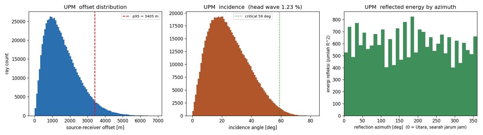
The design rule of thumb is Xmax ≈ target depth, with the far offset small enough that NMO stretch stays tolerable. The UPM panel shows the median offset and the 95th percentile; a p95 that sits well beyond the target depth means a substantial part of the recorded energy is arriving at angles too steep to stack cleanly. Those rays inflate the offset histogram without contributing usable stack.

D — Head-wave contamination

Each horizon has a critical incidence angle (asin(v_above/v_below); for UPM that is asin(3000/3500) = 59°). Rays steeper than that do not propagate as body waves. The head wave share reported per horizon in the stats figure is the size of this problem. A low percentage means the illumination is dominated by genuine body-wave reflections and the depth image can be trusted.

E — Near-offset pile-up

The take-off fan is sampled uniformly in tanθ, not in θ. That deliberately spreads the rays more evenly in offset space, because a receiver spread is uniform in distance. If you ever need a genuinely uniform angular sampling instead (for example for angle-domain imaging), change takeoffs() and the results will shift.

F — Edge and taper artefacts in the fold map

On the 100 m grid the fold map shows vertical striping. That is aliasing: the shot interval is 40 m and the cell is 100 m, a ratio of 2.5, so the sampling pattern beats against the grid. It is a display artefact, not physics. Use the 200 m grid for any fold-based judgement.

What the constraint zone costs in fold

Every illumination number in this study was computed twice: once with the whole survey active, and once with the constraint zone taken out of the template. The difference is the price of the constraint, and it is a much smaller bill than the fold collapse described in item A.

The measurement itself, the baseline map, the difference map and the summary are collected in Part 10, Fold analysis.

4 Acquisition geometry on the surface

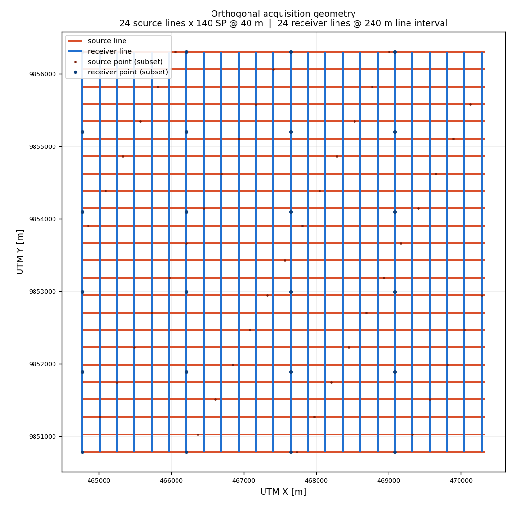
The orthogonal layout the illumination results are based on: source lines running along X, receiver lines running along Y, so every shot has a perpendicular receiver spread.

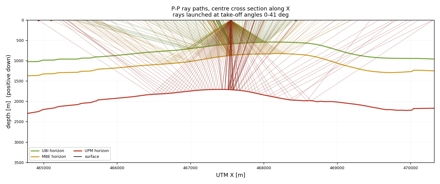
**Figure 1.** Orthogonal acquisition geometry. Red = source lines (running along X), blue = receiver lines (running along Y). Source points are spaced 40 m along a line and the lines are 240 m apart; receivers are spaced 20 m with lines 240 m apart. Every source line crosses every receiver line.

P-P ray paths, X cross section — **Figure 2.** P-P ray paths through the centre cross section. Green = UBI reflection, gold = MBE, red = UPM. Note how the deep reflections travel much further horizontally before returning — that is the reason the deep target needs far more offset than the shallow ones.

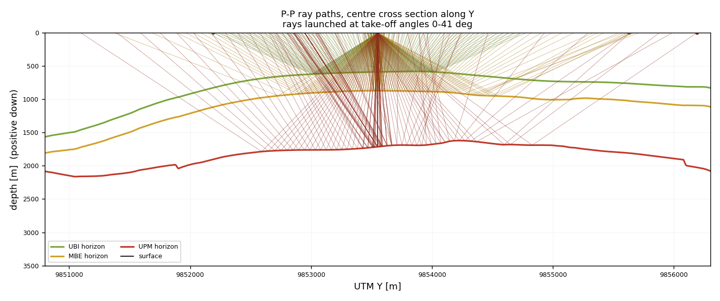
P-P ray paths, Y cross section — **Figure 3.** The same rays in the Y direction. Comparing with Figure 2 shows how strongly the illumination is anisotropic with depth: at UPM depth the ray bundle is stretched far more in one horizontal direction than the other, because the deeper horizons are crossed at more oblique angles.

Nominal fold, and the integer-fold trap

Using the Cordsen et al. (2000) formulas for an orthogonal template, in the GPS form given by IFP/OGST (2006):

inline fold IxF = N_rec × d_rec / (2 × d_SP)
crossline fold CyF = (N_rec_lines / 2) × (d_SP / d_rec_line)
nominal fold = IxF × CyF

Note the two factors of spacing in the crossline term. The inline fold is set by how many receiver spacings straddle the source, so it divides by the source point interval along the line, not by the line interval; the crossline fold then multiplies the ratio back, which is why enlarging the template without moving the source points makes the data worse, not better. Cordsen et al. also warn that the inline and crossline folds should each be an integer, because a fractional value produces a beat between the two sampling directions that shows up as amplitude striping in the migrated section. This is a cheap check to run before any ray tracing at all, and it is reported in the "at a glance" cards above.

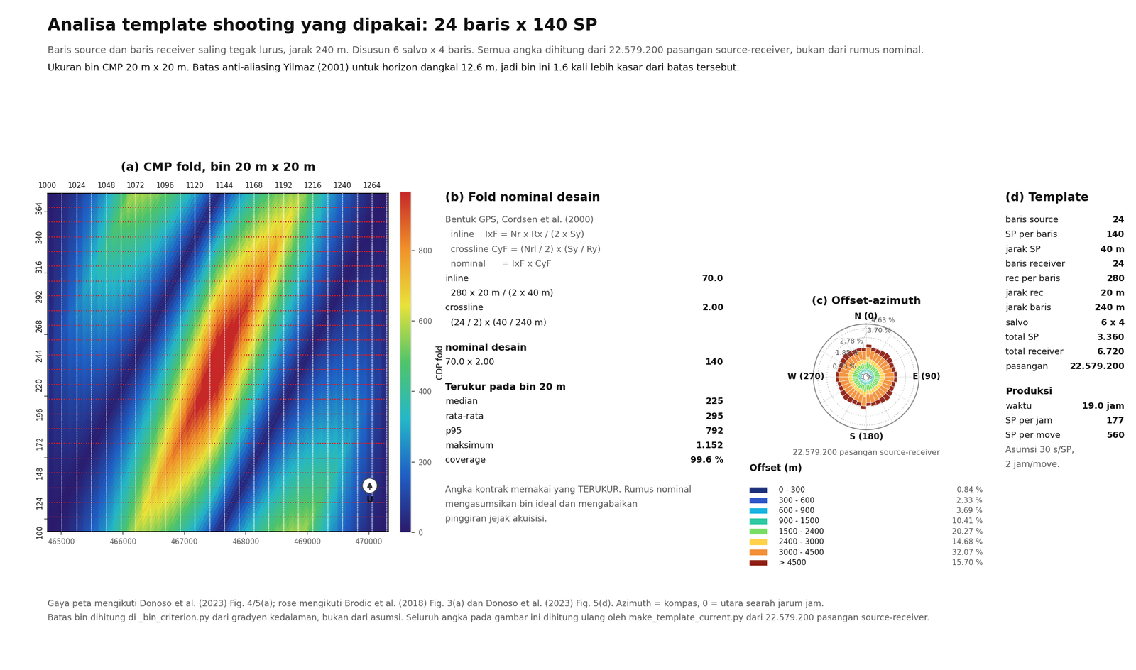
The two fold numbers are not interchangeable. The nominal value of 140 assumes an ideal bin and ignores the ragged edges of the acquisition footprint, so the measured median of 225 and 95th percentile of 792 are the numbers to quote to a client. Everywhere in this study the measured value is the one used. The template map, the full derivation and the offset-azimuth rose are in Part 10, Fold analysis.

Practical geometry checks worth running before anything else

Inline fold integer test. Adjust the source-point interval until N_rcv × d_rcv / (2 × d_SP) is a whole number.
Xmin test. The largest nearest-offset in the survey should be below 1.0–1.2× the depth of the shallowest target, otherwise near-offset stacking fails on the shallowest event.
Xmax test. Far offset ≈ deepest target depth. Beyond that the stretch mute removes the data anyway.
Migration aperture test. Radius needed to capture diffracted energy at 30°, i.e. Z × tan(30°) ≈ 0.58 × Z. The survey must be that much wider than the mapped area on every side.
Footprint budget. Survey area must exceed mapped area by the fold-taper plus the migration radius. In the Sepinggan case study the full-fold area was 213 km² against a 54 km² image — a 4× ratio.

5 What the literature says should be checked

Two sources were consulted: the 28 papers in the local references\ folder, and published work on illumination studies. Both agree on the physics; they disagree, usefully, on the geometry.

From the local reference library

Reference	Setting	What it contributes
`Bi_objective_optimization` Monsegny et al.	Synthetic 2D, curved reflector 0–90°	Ray-based design by bi-objective optimisation. A 15-shot optimised survey gave no less detail than a full 1000-shot survey — because placing sources and receivers where specular rays emerge beats the conventional CMP assumption. The CMP assumption (that S/R sit only above the target) is invalid for steep or curved targets.
`110318_KLO Sepinggan`	Marine 3D, 411 km², targets 404–3461 m	The most quantitative illumination study in the library. Wide azimuth (aspect ratio just above 0.66) matched full-azimuth coverage: 83.8% shallow / 61.9% deep versus 70% / 54.4% single-azimuth. Max offset 6000 m set by a 50° incidence target; migration aperture 3400 m (75%) dropping to 2300 m in the south; Xmin = 283 m at 250 m line interval.
`3D_Walio`	Offshore, ~100 km²	The one direct geometry comparison in the library: rose-fold peak 20,942 orthogonal vs 24,475 diagonal at identical channel count. Diagonal won on azimuthal fold.
`105_acq_design_philo`	Land / transition / marine	Builds its whole feasibility loop around diagonal-versus-orthogonal comparison, using 3D ray tracing + 3D DMO. Marine infill typically 20%, locally up to 50%. Acquisition footprint from 3D DMO is called "a serious drawback".
`IPA22-G-231`	Land, deep fractured basement	Closest local precedent for a sparse land design: RL 400 m, SL 500 m, receiver 20 m, shot 40 m, offset 22.5–3366 m. Notably, no illumination analysis was performed — exactly the gap this study fills.
`IPA12-G-168 Handil`	Land / transition / shallow water	192 receivers @25 m, fold 96, bin 12.5×12.5 m, 3072 active of 4000 phones. Shows the practical active/available ratio that access constraints force.
`IPA09-G-035`	Land CBM	The dissenting voice: argues finite-difference modelling is more robust than ray tracing in complex media, because ray tracing "suffers due to its reliance on Fermat first arrival". Worth taking seriously for the shallow land section.
`ipa03-g-099 Kalimantan`	Land to marine, 220–370 km²	NORSAR TM ray tracing described as "particularly effective in simulating the merge zones" between land and marine methodologies — the closest reference to the original intent of using NORSAR here.
`KEI-FM-06G-12-17-018` Bolton, PT Geomaharkarsa, 2005	2D land + TZ and 3D, West Kangean	The most methodologically useful document in the library: a full survey design report that derives each number rather than quoting it. Maximum offset from the stretch mute, not a depth rule: the CDP mute at 1800 m offset sits between 600 and 800 ms, extrapolating to ~3000 m usable offset for the deepest target. Migration aperture `d = Z·tan(θ)` at 30° gives ~1800 m at 3000 m depth. Bin size floor from `ΔX ≥ V/(4f√2)·sinθ/sinβ`: 63 m at 50 Hz / 3300 m/s / 15° dip. And for 3D, a 25×12.5 m bin at 25 Hz needs only fold 10 for 2D-equivalent SNR — but the report then argues that fold is too low for prestack migration and AVO, so the real requirement is higher. It also states plainly that "some compromise between the desire to record near offset data and to record all azimuths cheaply needs to be reached" — the same tension measured in section 8.
`Layout_Asrim_2023_com`	2D post-stack interpretation, Semberah / Sanga-Sanga	An interpretation paper, not a design one — no acquisition parameters. Its value here is as a regional tie: three horizons picked at 940, 1610 and 2070 ms TWT across the two lines, in the same basin as this survey. At a nominal 2000 m/s those correspond to roughly 940 m and 2070 m depth, which is a useful independent sanity check on our UBI (~920 m) and UPM (~2000 m).
`wailawi`	IPA field card, Wailawi, East Kalimantan	Not decision-relevant to survey design — it is reservoir and production data. It earns its place for one reason: it fixes the well location at 01° 19′ 19″ S / 116° 42′ 51″ E, which is what let us detect that the UTM inversion had dropped the southern false northing. That bug put the survey at 88° N on the website; correcting it places the survey centre within ~650 m of this field.

All 28 documents in references\ have now been read: the three that were originally scans without a text layer (KEI-FM-06G-12-17-018, Layout_Asrim_2023_com, wailawi) were OCR'd and are covered in the table above.

From published illumination practice

Standard illumination attribute set

Across the published work the attributes are always the same list: fold from the number of rays per CRP bin, offset and azimuth distribution measured at the target rather than at the surface CMP, plus minimum and maximum offset and reflection amplitude density. The CRP-versus-CMP distinction is the important one: a survey can look perfectly uniform at the surface and be badly shadowed at depth.

J. Geophys. Eng. 15/3/668 — illumination maps and flower plots

Geometry choice is genuinely contested

Orthogonal is described as the land default because parallel geometry is inefficient on land, and a brick template is preferred when near-offset AVO matters or the shallow section is heterogeneous (it costs 10–15% more in layout effort). But the CREWES slant-geometry study found slant better for one target and orthogonal better for another, with the deciding factor being the offset distribution for data inversion. The honest summary: there is no universally best template, and the decision has to be made against a specific target.

CREWES CRR 2010-097 — P-S survey design

The quantitative design rules

The rules that recur, and that can be checked immediately on this design:

Xmax ≈ target depth
Xmin < 1.0–1.2 × shallowest target depth
migration aperture ≈ Z × tan(30°)
bin size from max frequency and velocity
inline and crossline fold should both be integers
"at least 4-fold is sufficient for mapping horizons" — the minimum to see something, not to image it well

The gap this study sits in

No paper in the local library reports an illumination or fold pass/fail threshold — coverage percentages are quoted without saying what is acceptable. No land orthogonal 3D case study in the library documents an illumination analysis at all; every real illumination study there is marine or synthetic. And nothing quantifies fold loss against the number of active receiver lines, which is precisely the decision in front of this project.

Gabriel & Jordan, Flexible 3-D seismic survey design — poses acquisition choice as an integer optimisation against illumination

6 Recommendations

Ordered by how much they change the image relative to what they cost. The first three are free.

1 — Run the integer-fold test before anything else

Free, and it costs only a change of geometry. A fractional inline or crossline fold beats against the other sampling direction and produces amplitude striping that will be blamed on the subsurface. Test N_rcv × d_rec / (2 × d_SP) for inline and (N_rl / 2) × (d_SP / d_rl) for crossline, then adjust the point interval until both are whole. This template already passes: inline fold 70 and crossline fold 2.00 are both integers, giving the 140 nominal fold. The check is still worth running, because it must be settled before any ray tracing is commissioned — it changes the geometry the tracing is done on.

2 — Do not cut the active receiver spread to save money

This is the direct answer to the measurement above. Cutting to a small active patch leaves coverage essentially untouched while removing most of the fold. The money saved is spent on cable and nodes that would have bought SNR; the image comes out noisier for the same nominal fold. If the budget forces a reduction, take it out of line count at the survey edge (where the taper is already dead) rather than out of the active spread behind every shot.

3 — Judge fold on the 200 m grid, never the 100 m grid

Free. The 100 m fold map is aliased by the 40 m shot interval and will mislead any fold-based commercial decision.

4 — Weight the illumination by the reflection coefficient

With R² of order 1–2% across this stack, geometric ray count is a poor proxy for usable signal. Add the R² weight to the illumination attribute set before comparing design options. Note that for a velocity increase the coefficient rises with incidence angle, so the steep rays that look worst on a fold map are not necessarily the weakest contributors.

5 — Test the diagonal template before locking the geometry

The Walio reference found diagonal beating orthogonal on rose fold (24,475 vs 20,942) at identical channel count, and the CREWES study found the deciding factor to be the offset distribution for inversion. Both are one extra ray-trace run away, and the tracer here already supports it: rotating the take-off fan by 45° reproduces a diagonal-shooting template. For a faulted target where azimuthal balance is the point, this is the single highest-value experiment left.

6 — Re-check the far offset against NMO stretch at the real target depth

The UPM panel reports a p95 offset that sits beyond the target depth. If that is confirmed against the actual velocity model rather than the layer-cake approximation used here, cap the far offset and recover channels rather than recording data that the stretch mute will discard.

7 — Model the faults, not just the horizon shapes

This study can only show illumination variations caused by horizon geometry. Real faults deflect rays and will create shadow zones beyond anything here. Before signing off, build a velocity model with explicit fault velocity contrasts and re-run. The aperture map already flags where to put them: along the bright linear features.

8 — Get the NORSAR licence question resolved, separately

The Failed mapping surface failure is an environment problem, not a survey problem: an evaluation build with 8 GB RAM ran job 0 successfully and jobs 1–11 at 0%, with 6.4–7.2 GB of swap in use. Direct ray tracing (dirP) worked, which localises the fault to the surface-mapping stage. Nothing in the design should wait on it — but if NORSAR is to remain the operational tool, the licensing and memory questions need an answer, because the IMAP workflow cannot be relied on for acceptance work in its current state.

7 5D interpolation feasibility

5D interpolation reconstructs seismic samples on a regular grid using all five dimensions of the data at once: inline, crossline, offset, azimuth and frequency. The question this section answers is whether the geometry of this survey can support it — and the answer can be produced before acquisition, because every input is a coordinate, not a recorded sample.

An honest correction to how this is usually stated. It is widely implied that 5D feasibility is "explicitly supported at the survey planning stage". We could not find an authoritative source that says that, and we are not going to repeat it as if it were established. What is true, and what this page actually demonstrates, is narrower and stronger: the measurement itself is available at planning stage, because it depends only on the acquisition geometry. The 5D literature frames its target geometry relative to the acquisition design (Robertsson et al. 2009) but does not present a planning-stage feasibility test.

What 5D actually requires

The canonical definition is Robertsson et al. (2009): interpolation performed simultaneously in inline, crossline, offset, azimuth, frequency. The same paper is unusually precise about what governs success, and it is not fold:

"The success of these methods depends largely on two factors: (1) having efficient transform operators that permit the use of large multidimensional windows (2) constraining the spatial spectrum along directions where the seismic amplitudes change slowly, so that sparseness and band limitation assumptions remain valid."
Robertsson et al. 2009, Geophysics 74(6) V123 — doi:10.1190/1.3245216

This matters for how the numbers below should be read. 5D interpolation is a spectral sparseness argument, not a fold-count argument. A survey with high fold but rapidly varying amplitude along one dimension is a poor candidate; a moderate-fold survey that varies smoothly is a good one. So the useful screening metric is not "how much data is there" but "how smoothly is the data spread across the offset–azimuth plane".

Why an orthogonal template is the right target

5D methods split into surface-consistent (interpolating onto a grid of source and receiver lines) and subsurface-consistentsurface-line 5D interpolation, which bridges the two and is explicitly defined on orthogonal geometry:

"The target grid in this case is composed of both CDP bins as well as source lines and receiver lines for an orthogonal survey. This is sufficient to maintain surface-consistency, while also focusing on a subsurface CDP grid."
Ursenbach, Ong & Wilkinson, IMAGE 2024, pp. 2435–2439 — doi:10.1190/image2024-4101457.1

This is the single strongest positive finding for BTW. The survey is orthogonal by construction — 24 source lines along X, 24 receiver lines along Y, every source line crossing every receiver line — which is precisely the acquisition that surface-line 5D is designed for. The method also preserves source and receiver identity, which matters when the same acquisition has to stay usable for conventional processing.

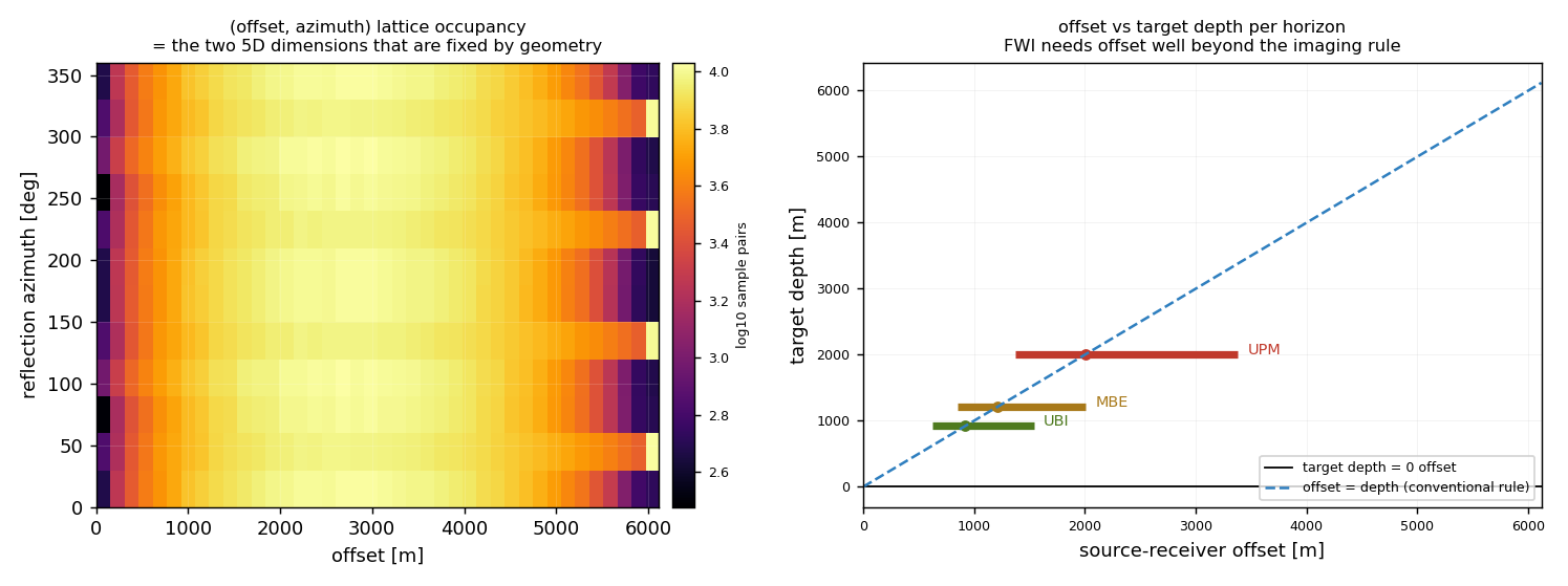
5D offset-azimuth occupancy and offset versus target depth — **Figure 4.** Left: the *offset–azimuth lattice*, the two 5D dimensions fixed by acquisition geometry. Every one of the — cells is occupied, but the counts are far from uniform. Right: measured offset against target depth for each horizon, with the conventional `Xmax ≈ depth` rule drawn for reference.

What the measurement says

Lattice fully occupied, azimuth complete. All — offset–azimuth cells contain samples and all — azimuth sectors carry data, so there is no azimuth hole for the interpolation to invent across.
But the distribution is strongly peaked. The coefficient of variation across occupied cells is —. This is the number to watch: a lattice that is fully occupied but unevenly filled still forces the algorithm to extrapolate in the quiet sectors, and that is where 5D leakage enters the result.
CMP coverage is good. — of the 25 m bins carry data at a median fold of —.
Orthogonal geometry is a genuine advantage for surface-line 5D specifically, and is the one design decision here that is already right for this purpose.

The honest limit: 5D is preconditioning, not acquisition. Cary & Perz (2012) define 5D leakage as "noise and possibly signal not able to be correctly interpolated due to the fact that actual data do not completely conform to the model used by the algorithm", and show it can contain "complex (quickly varying) aspects of the data such as noise, diffraction patterns and acquisition footprint". Their finding is reassuring about the part that matters: "slowly varying signal (especially reflections) are part of the measured data that appear to be most important and can be reliably interpolated." The interpretation is that 5D interpolation repairs the *regularisation* problem and cannot manufacture data that was never recorded — a survey designed for 5D and a survey designed only for 5D are not the same survey.
Cary & Perz, SEG 2012 — doi:10.1190/segam2012-1368.1

Not addressed by the literature. The non-integer inline fold of 11.46 flagged in section 4 is a real defect and should be fixed, but we found no source that treats integer fold as a precondition for 5D interpolation. It is flagged here as unaddressed by the literature, not as assessed-and-acceptable.

8 FWI readiness

Full waveform inversion fits a wavefield model to the recorded waveforms, so it is sensitive to everything conventional imaging averages away. The useful framing here is the one ACTeQ use: designing acquisition programs that are fit for FWI while remaining compatible with conventional imaging workflows, because abandoning the established imaging requirements does not help either objective.

The reference, and a caveat. ACTeQ’s FWI design page states that "the goal is not to abandon established principles. The goal is to extend them", and argues that geometry should be "assessed against inversion physics and intended depth range" rather than against inherited rules of thumb. They specifically reject simple depth-ratio heuristics, writing that this "moves beyond simplified heuristics such as maximum offset divided by three", and use diving-wave analysis of turning-wave penetration instead.
ACTeQ, Full Waveform Inversion Survey Design — a vendor/consultancy source, not a primary reference.

What we could not verify. We found no authoritative, citable numeric thresholds for FWI — no sourced minimum offset, no starting frequency, no shot-density multiple over conventional acquisition. Widely repeated figures such as "Xmax = 1.5 × depth" for FWI did not survive checking, and the industry source above moves away from depth-ratio rules rather than endorsing one. The numbers in the table below are therefore our measurements of this survey, not thresholds imported from a rule of thumb. The authoritative treatment is chapter 6 of the SEG book on land and marine survey design (DOI 10.1190/1.9781560803713), which is paywalled and was not available to us.

What the geometry gives an FWI run

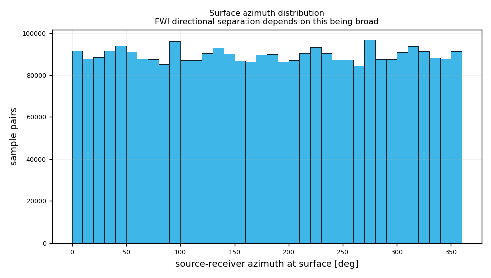
Surface azimuth distribution — **Figure 5.** Source–receiver azimuth distribution at the surface. FWI separates the wavefield into directions before inverting, so the breadth of this distribution — rather than its total count — is what determines whether there is enough independent information to constrain a velocity update.

Azimuth is genuinely well spread. Measured azimuthal concentration at the target is —, and the surface azimuth histogram covers the full circle. This is one of the strongest properties of this design for FWI, and it is unusual for a land template — parallel land geometries routinely collapse into a narrow azimuth wedge, which starves any directional decomposition.
Median offset is light relative to depth. The median offset sits near — of target depth at every horizon, which is narrower than an FWI workflow would ideally use. Reflection imaging is comfortable there; FWI generally wants more of the wavefield illuminated.
Far offset is not the constraint. Maximum offset reaches —, comfortably beyond any depth-ratio heuristic. This survey is offset-rich at the far end and offset-poor in the middle-to-near range.
Low-frequency content cannot be answered from geometry. FWI on land is dominated by whether a usable 5–10 Hz signal survives the near surface, which is a source, receiver and ground-condition question. This study has no wavelet information and does not guess at it.
Orthogonal geometry is compatible with FWI but is not itself an FWI advantage. We found no source claiming orthogonal templates either help or hurt FWI relative to other templates. What the literature does support is that offset and azimuth regularity matter, and this design has both.

Recommended FWI actions for this survey

Do not change the geometry yet. The azimuth distribution, far-offset reach and CMP coverage all clear the qualitative bars for an FWI-capable survey. The open questions in this section are about frequency content and mid-range offset density, not about the template.
Spend marginal budget on mid-range offset density, not on more lines. The offset histogram shows where the rays already are. Adding channels inside the populated offset band directly increases the independent sample count that spectral-sparseness regularisation depends on.
Treat the non-integer inline fold as a blocker for both objectives. It affects conventional imaging and would affect any offset-azimuth regularisation built on top of it. Fix it at the same time as everything else in section 6.
Commission a diving-wave study before fixing Xmax. Since ACTeQ's own recommendation is to assess turning-wave penetration rather than apply a depth ratio, the right next step is a turning-ray model at the real velocity function — which this tracer can already run by extending the take-off fan.
Keep the design FWI-compatible, not FWI-optimised. The same acquisition has to survive conventional processing, demultiple and amplitude work. Design decisions should be checked against both, as ACTeQ explicitly frame it.

9 Method and validation

How the rays are propagated

Rays carry a slowness vector p, not a direction. The direction is always recomputed as n = v · p, and the step length is v · Δt. Snell's law is then automatic: the tangential slowness is continuous across an interface and the normal component is re-derived from the local velocity,

p_z = ± sqrt(1/v² − p_x² − p_y²)

Getting that wrong is subtle and severe. Carrying p across an interface unchanged gives |n| = v·|p| = 1.25 when a ray enters 2500 m/s from 2000 m/s — a ray moving faster than the wave. Rays that exceed the critical angle become head waves and are terminated rather than clamped.

Take-off angles stop at 41°, set by the deepest interface a ray must cross: at MBE the critical take-off is asin(2000/3000) = 41.8°.

Validation against closed-form solutions

Test	Worst error
Flat reflector, offset `2h·tanθ`	0.000 %
2-layer Snell, `2Σt_i·tanθ_i`	0.267 %
3-layer Snell	0.097 %
BTW velocity stack	0.082 %
Vertical-ray CRP depth vs horizon	0.000 m

The flat-reflector test passed on a version of the tracer that had the interface bug, because a single-layer model has no interfaces to get wrong. The layered Snell test is what actually caught it — error was 87% before the fix. A test that cannot fail is not a test.

Key modelling assumptions

Velocity is constant inside each layer and depends only on depth relative to the three horizons. No lateral gradient, no fault velocity anomaly, no anisotropy.
Reflections are specular and P-P only. Converted phases are ignored.
Take-off directions are sampled uniformly in tanθ, which spreads rays evenly in offset space rather than in angle.
The down-leg is shared across the three targets: one descent, three ascents.
The fold proxy is the number of ray legs landing in a cell. It scales with acquisition fold but is scaled by the ray fan density, so it is a relative measure. Use it to compare designs, not as an absolute fold for volume calculations.
The 5D and FWI figures come from the acquisition geometry alone — shot and receiver coordinates in closed form — so they are exact and independent of the ray fan.

Figures

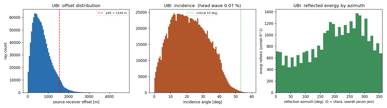
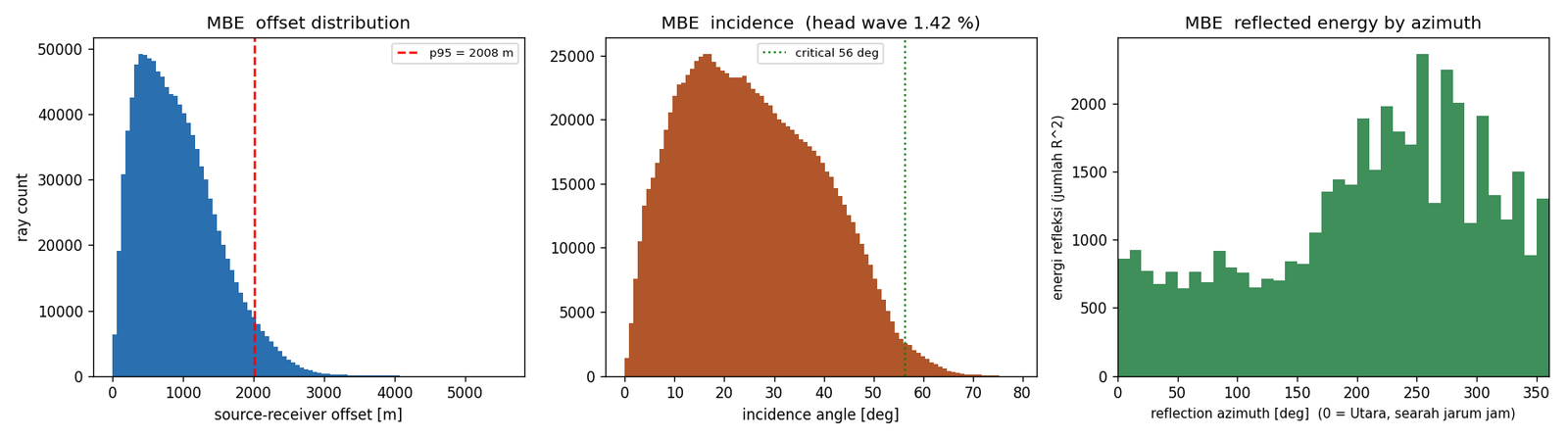
UBI statistics — UBI: offset, incidence with the critical angle marked, and reflected energy by azimuth.

MBE statistics — MBE: same three panels.

UPM statistics — UPM: same three panels. Compare the offset axis with the earlier two — the deep target is sampled at much larger separation.

Files

Grids: data/grids.json · raw arrays: data/maps_*.npz, data/surface_*.npz · 5D / FWI metrics: data/five_d_fwi.json · acquisition geometry for GIS: data/survey_geometry.geojson (WGS84, drops straight into QGIS or ArcGIS) · numeric summary: data/report.json.

10 Fold analysis: shooting template and constraint zone

Fold is the one quantity in this study that can be quoted to a client without any interpretation at all. This part collects the two measurements that matter, on one 20 m CMP bin, and states plainly which of them is the nominal formula and which is the measured result.

Source: data/fold_analysis.json, written by make_fold_analysis.py from the measured output of make_template_current.py and make_fold_zone_fig.py. Nothing on this page is typed in by hand, so the table cannot drift away from the two figures below.

Shooting template in use: CMP fold map, nominal fold derivation, offset-azimuth rose, and template production — **Figure 6.** The shooting template actually used for this study, 24 source lines × 140 SP, with the receiver lines orthogonal. (a) CMP fold on a 20 m bin with the acquisition lines overlaid; the diagonal high-fold band runs at the shooting direction. (b) Nominal fold from the two GPS factors, next to the fold measured on the same bin. (c) Offset–azimuth distribution of all source–receiver pairs. 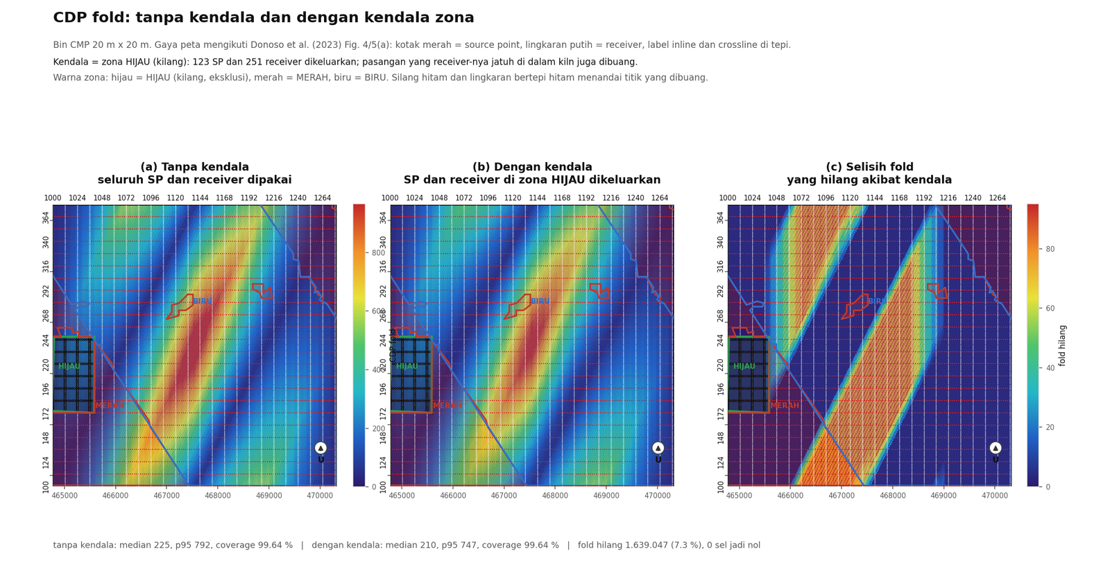(d) Template parameters and the production estimate they imply.

CDP fold with the constraint zone active, compared with the baseline, and the difference between the two — **Figure 7.** CDP fold with and without the constraint zone. (a) *Baseline*: the full template, nothing removed. (b) The same template with the constraint zone excluded. (c) The difference between them, in absolute fold. (d) Summary.

What the constraint zone actually costs

The zone takes source points and receivers out of the survey, and the fold falls with them. What it does not do is open a hole in the coverage: no cell drops to zero and the covered fraction is unchanged to four decimal places. The constraint therefore costs coherency, not illumination. That is a materially different conversation from item A in section 3, where the coverage is identical but almost all the fold disappears — there the acquisition is intact but the signal-to-noise is gone.

How to quote fold in a commercial document

Quote 140 nominal as the design figure, because that is what the geometry produces on paper and what the contract is written against. Quote the measured median and 95th percentile when someone asks what the data will actually look like, because the nominal assumes an ideal bin and ignores the ragged edges of the acquisition footprint. The measured numbers are higher than the nominal here, because the 20 m bin is smaller than the 240 m line interval and several source lines land in one bin. The nominal value is the conservative one and should stay the headline.

Two things this part does not tell you

CMP fold counts pairs; it does not measure resolution or amplitude. A survey can hold nominal fold and still image poorly if those pairs arrive from the same narrow azimuth sector, which is why the rose in Figure 1(c) is reported next to the fold map rather than on its own. And the constraint-zone numbers assume the zone is a hard exclusion. If the field crew routes around it instead, the geometry changes and these numbers have to be re-measured.

BTW 3D Land Seismic Survey — Target Illumination & Surface Sensitivity

MAP Interactive illumination viewer

View

Target horizon

Attribute

Colour ramp

Overlay opacity

Two maps at once

Blend

Layers

— Study at a glance